Assessment
Accreditation period Units 1-4 from 2023
General assessment advice
Advice on matters related to the administration of Victorian Certificate of Education (VCE) assessment is published annually in the VCE Administrative Handbook.
Updates to matters related to the administration of VCE assessment are published in the VCAA Bulletin.
Teachers must refer to these publications for current advice.
The principles underpinning all VCE assessment practices are explained in VCE assessment principles.
The glossary of command terms provides a list of terms commonly used across the Victorian Curriculum F–10, VCE study designs and VCE examinations and to help students better understand the requirements of command terms in the context of their discipline.
VCE Mathematical Methods examination specifications, sample examination papers and corresponding examination reports can be accessed from the VCE Mathematical Methods examination webpage.
Graded distributions for graded assessment can be accessed from the VCAA Senior Secondary Certificate Statistical Information webpage.
Excepting third-party elements, schools may use this resource in accordance with the VCAA’s educational allowance (VCAA Copyright and Intellectual Property Policy).
Scope of tasks
For Units 1–4 in all VCE studies, assessment tasks must be a part of the regular teaching and learning program and must not unduly add to the workload associated with that program. They must be completed mainly in class and within a limited timeframe.
Points to consider in developing an assessment task:
- List the relevant content from the areas of study and the relevant key knowledge and key skills for the outcomes.
- Develop the assessment task according to the specifications in the study design. It is possible for students in the same class to undertake different tasks, or variations of components for a task; however, teachers must ensure that the tasks or variations are comparable in scope and demand.
- Identify the qualities and characteristics that you are looking for in a student response and map these to the criteria, descriptors, rubrics or marking schemes being used to assess level of achievement.
- Identify the nature and sequence of teaching and learning activities to cover the relevant content, and key knowledge and key skills outlined in the study design, and to provide for different learning styles.
- Decide the most appropriate time to set the task. This decision is the result of several considerations including:
- The estimated time it will take to cover the relevant content from the areas of study and the relevant key knowledge and key skills for the outcomes
- The possible need to provide preparatory activities or tasks
- The likely length of time required for students to complete the task
- When tasks are being conducted in other studies and the workload implications for students.
Units 1 and 2
The students' level of achievement in Units 1 and 2 is a matter for school decision. Assessments of levels of achievement for these units will not be reported to the VCAA. Schools may choose to report levels of achievement using grades, descriptive statements or other indicators.
In each VCE study at Units 1 and 2, teachers determine the assessment tasks to be used for each outcome in accordance with the study design.
Teachers should select a variety of assessment tasks for their program to reflect the content and key knowledge and key skills being assessed and to provide for different learning styles. Tasks do not have to be lengthy to make a decision about student demonstration of achievement of an outcome.
A number of options are provided to encourage use of a range of assessment activities. Teachers can exercise flexibility when devising assessment tasks at this level, within the parameters of the study design.
Note that more than one assessment task can be used to assess satisfactory completion of each outcome in the units, and that an assessment task can typically be used to assess more than one outcome.
There is no requirement to teach the areas of study in the order in which they appear in the units in the study design. In mathematics an activity or task will often draw on content from one or more areas of study in natural combination, and involve key knowledge and skills form all three outcomes for the study.
Unit 1 sample assessment tasks
Sample investigation: Exploring long run probabilities
Sample investigation: Exploring long run probabilities
The investigation is to be conducted over a period of about 1 week.
Introduction
This task involves students predicting the number of trials required before experimental results closely align with the expected long run probabilities.
Students then conduct a random experiment to test out their prediction and use a technology-based pseudo-random simulation to compare outcomes with expected long run probabilities.
Equipment: Each student will need four different coloured six-sided dice.
Formulation
Overview of the context or scenario, and related background, including historical or contemporary background as applicable, and the mathematisation of questions, conjectures, hypotheses, issues or problems of interest.
The expected long run probability of each number being rolled on a fair six-sided dice is.
Students are to predict the number of trials required of rolling a fair six-sided dice before experimental results start to closely match the expected long run probability, explaining their reasoning and listing any assumptions made.
Exploration
Investigation and analysis of the context or scenario with respect to the questions of interest, conjectures or hypotheses, using mathematical concepts, skills and processes, including the use of technology and application of computational thinking.
Part 1:
Roll four six-sided dice simultaneously at least 150 times, recording the results and graphing the corresponding distribution.
Part 2:
To enable analysis of experimental results representing a range of total number of rolls, collate and compare the results as follows:
- for each of the four six-sided dice
- combined total of their four six-sided dice results
- combined total of their and nine other students' step b. results.
Analyse the results in steps a. to c. by calculating the percentage difference between the experimental results and the expected long run probabilities for a suitable level of accuracy, and consider how these results compare to the initial prediction.
Part 3:
Use technology to simulate the pseudo-random rolling of a fair six-sided dice to determine the number of trials required before the simulated outcomes and the expected long run probabilities match the level of accuracy used previously.
Communication
Summary, presentation and interpretation of the findings from the mathematical investigation and related applications.
Summarise findings and compare and interpret them in relation to the initial prediction made.
Describe the relation between the experimental probability and the expected value.
Areas of study
The following content from the areas of study is addressed through this task.
| Unit 1 | |
| Area of study | Content dot points |
| Functions and graphs | – |
| Algebra | – |
| Calculus | – |
| Probability and statistics | 1, 2 |
Outcomes
The following outcomes, key knowledge and key skills are addressed through this task.
| Outcome | Key knowledge dot points | Key skills dot point(s) |
| 1 | 9, 10 | 16 |
| 2 | 1, 2, 3, 5 | 1, 2, 3, 5, 6 |
| 3 | 1, 7, 8 | 1, 2, 4, 5, 10, 12, 13 |
Sample investigation: Implementing the bisection algorithm with polynomial functions
Sample investigation: Implementing the bisection algorithm with polynomial functions
This investigation is to be conducted over a period of about 1 week.
Introduction
A context such as the following could be used to develop a mathematical investigation that applies the three investigation components of formulation, exploration and communication to connect several aspects of the mathematics of polynomial functions. These include remainder, factor and rational root theorems. The application of the numerical method of the bisection algorithm for approximating irrational real roots of these functions.
The bisection algorithm is a bracketing method and examples of implementation can be found online.
Formulation
Overview of the context or scenario, and related background, including historical or contemporary background as applicable, and the mathematisation of questions, conjectures, hypotheses, issues, or problems of interest.
In this task, formulation is related to the statement of theorems, selection and variety of functions, how the description will be represented and implemented as an algorithm, and questions for analysis.
Exploration
Investigation and analysis of the context or scenario with respect to the questions of interest, conjectures, or hypotheses, using mathematical concepts, skills, and processes, including the use of technology and application of computational thinking.
In this task, exploration is related to application of theorems and analysis of related examples for selected polynomial functions, the application of the algorithm using technology, and the systematic analysis of results, including consideration of accuracy.
Communication
Summary, presentation, and interpretation of the findings from the mathematical investigation and related applications
In this task, communication is related to the summary of results for the functions involved, and discussion of the terminating conditions for the algorithm with respect to the accuracy of the approximate solutions for roots.
Part 1
- State the remainder, factor, and rational root theorems, and give an example of their application to each of a quadratic, cubic and quartic polynomial function, for cases where a rational root exists, and for cases where a rational root does not exist.
- Use a suitable selection of graphs to show that a quadratic function can have 0, 1 or 2 real roots, a cubic polynomial function can have 1, 2 or 3 roots, and a quartic polynomial function can have 0, 1, 2, 3 or 4 real roots.
- Explain why a cubic polynomial function must have at least one real root.
Part 2
- Explain how the bisection algorithm works and show how it is implemented by the technology that is being used.
- Apply the bisection algorithm to determine point estimates for the non-rational real roots of a quadratic function, a cubic function, and a quartic function.
- Investigate the effect of the terminating condition on the accuracy of the approximation with respect to the number of iterations required.
Areas of study
The following content from the areas of study is addressed through this task.
| Area of study | Content dot point(s) |
| Functions and graphs | 4 |
| Algebra | 1, 2, 6, 7 |
| Calculus | |
| Probability and statistics | - |
Outcomes
The following outcomes, key knowledge and key skills are addressed through this task.
| Outcome | Key knowledge dot points | Key skills dot points |
| 1 | 1, 10, 12 | 7, 10, 11, 12, 13 |
| 2 | 1, 2, 3, 4, 5 | 2, 3, 5, 6 |
| 3 | 1, 2, 5, 6, 7, 8 | 1, 3, 4, 5, 7, 9, 10, 11, 12, 13 |
Sample context for assessment: Investigating different approaches to solving quadratic equations
Sample context for assessment: Investigating different approaches to solving quadratic equations
Introduction
There are several approaches that can be used to solve quadratic equations of the form ax2 + bx + c = 0 or equivalent equations. These may provide exact or approximate solutions for one or both roots, where these exist, depending on the context.
The investigation below considers several of these approaches and their application to solving quadratic equations. An assessment task could comprise a selection of parts of the task. Note that some introductory work on calculus would need to have been completed prior to undertaking Part 5.
Part 1: The quadratic formula
- State and derive the quadratic formula.
- Verify that the formula is true.
- Explore what happens for the cases b = 0, c ≠ 0, b ≠ 0, c = 0 and b = c = 0.
Part 2: Alternative version of the quadratic formula
There is an alternative quadratic formula: $$x = $\Large\frac{2c}{-b \mp \sqrt{b^2 - 4ac}}$$
- Use a range of examples to verify that this alternative formula gives the same solutions as the usual quadratic formula.
- Derive the alternative version of the quadratic formula.
- Show that the two quadratic formulas are equivalent.
Part 3: Comparing the formulas – numerical computations
Compare the standard and alternative quadratic formulas with respect to numerical values obtained for various combinations of a, b and c and the separation of the two roots.
Part 4: Exact values, some estimates and approximations
- Plot the graph of f(x) = x2 - 2x - 1 on a one-to-one axes scale over a suitable interval and use the graph to estimate the location of the two roots of the function.
- Use the rational root theorem to explain why there is no rational root.
- Use a table of values to determine the approximate values of the roots correct to two decimal places.
- Complete the square to find the exact solutions to x2 - 2x - 1 = 0, and use compass and straight edge construction to locate the roots exactly on the graph.
- Use bisection to find an approximate value for the positive root.
- Show that x2 - 2x - 1 = 0 is equivalent to $$\large x = 2 + \frac{1}{x}, \quad x \ne 0$$
- Consider the equivalent form of the equation as a recurrence relation $$\large x_{n+1} = 2 + \frac{1}{x_n}$$ initial value x0 = 3. Implement this using technology to calculate the sequence {x1,x2,x3,...,x10}.
- Explore what happens for different values of x0.
- Use the positive root to find an approximate value for the other root.
Part 5: Newton's method (extension)
- Use a combination of pseudocode and technology to implement Newton's method to solve x2 - 2x - 1 = 0 with initial value
x0 = 3.
Plot the graph of the function and the first two tangents on the same set of axes using a one-to-one axes scale.
- Explore how Newton's method behaves for this equation for different initial values.
- Apply Newton's method to find an approximation for $\sqrt{20}$ and several other irrational square roots.
- The ancient Babylonians used a process for finding the square root of a positive integer, s, that can be represented in modern notation by the formula:
$$\large x_{n+1} = \frac{1}{2} \left( x_n + \frac{S}{x_n} \right)$$
Use Newton's method to derive this formula.
Areas of study
The following content from the areas of study is addressed through this task.
| Unit 1 | |
| Area of study | Content dot point(s) |
| Functions, relations and graphs | 3 |
| Algebra, number and structure | 1, 2, 3, 4, 5, 6, 7 |
| Calculus | 3 |
| Data analysis, probability and statistics | – |
Outcomes
The following outcomes, key knowledge and key skills are addressed through this task.
| Unit 1 | ||
| Outcome | Key knowledge dot points | Key skills dot points |
| 1 | 1, 2, 6 | 2, 3, 4, 5, 7 |
| 2 | 1, 2, 3, 4, 5 | 1, 2, 3, 5, 6 |
| 3 | 1, 2, 3, 4, 5, 7 | 1, 2, 3, 4, 6, 10 |
Sample context for assessment: Scaling human measures
Sample context for assessment: Scaling human measures
Introduction
This task uses a simple model of a human body to explore the effects of scaling linear dimensions on surface area and volume. Related topics in the application of mathematics in biology are allometry, power laws, the square–cube law, isometric scaling, geometric similarity and biomechanics.
Part 1
Consider a cube:
- Plot the graphs of surface area and volume as functions of side length, for side lengths from 0 cm to 100 cm in steps of 10 cm.
- Plot the graph of side length as a function of surface area, for surface area from 0 to 6 square metres.
- Plot the graph of side length as a function of volume, for volume from 0 to 1 cubic metre.
- Provide several examples of calculations that show how to determine a side length that would produce a specified surface area or volume.
Part 2
Consider a sphere:
- Plot the graphs of surface area and volume as functions of radius, for radii from 0 cm to 50 cm in steps of 10 cm.
- Plot the graph of radius as a function of surface area, for surface area from 0 to 4 square metres.
- Plot the graph of radius as a function of volume, for volume from 0 to 1 cubic metre.
- Provide several examples of calculations that show how to determine a radius that would produce a specified surface area or volume.
Part 3
A rough model of the human body can be made by considering the arms and legs as cylinders, the torso as a rectangular prism and the head as a sphere.
- Using reasonable approximate measurements from a friend, form such a model, specify the relevant linear dimensions in centimetres and calculate the surface area in square centimetres and volume in cubic centimetres for this model.
- Consider scaling factors for a similarity transformation (dilation) of linear dimensions from 0.1 to 2 in steps of 0.1. Plot a graph of surface area in terms of scaling factor and a graph of volume in terms of scaling factor.
Part 4
Investigate examples of large statues throughout history, such as the Colossus of Rhodes, and the biomechanics of bone strength and mass under scaling.
Areas of study
The following content from the areas of study is addressed through this task.
| Unit 1 | |
| Area of study | Content dot points |
| Functions and graphs | 1, 2, 3 |
| Algebra | 1, 2, 4, 5 |
| Calculus | – |
| Probability and statistics | – |
Outcomes
The following outcomes, key knowledge and key skills are addressed through this task.
| Unit 1 | ||
| Outcome | Key knowledge dot points | Key skills dot points |
| 1 | 1, 2, 3, 4, 5 | 1, 2, 3, 11, 13, 14 |
| 2 | 1, 2, 5 | 1, 2, 3, 5, 6 |
| 3 | 3, 4, 5, 8 | 3, 5, 6, 7, 12, 13 |
Sample context for assessment: Features of graphs of functions from data
Sample context for assessment: Features of graphs of functions from data
Introduction
This short task has two parts, both based on identification and analysis of features of graphs of functions. The functions involved represent real-life data and are not specified by a rule. Students are asked to use the graph to identify:
- Domain, range and co-domain for the function
- Points corresponding approximately to local and global maxima and minima, where there is sudden change and where the function has a specified value
- Approximate intervals corresponding to subsets of the domain over which the function is steady, increasing, decreasing, above, below or between specified values
- Other features of the function.
Part 1
Consider the function represented by the following smoothed trend graph, which shows the exchange rate between Australian and United States (US) dollars over the course of about a month (source: Exchange Rates | RBA).
- State the domain and range and a suitable co-domain.
- State the coordinates of any local maximum or minimum values.
- State the coordinates of the global maximum and the global minimum.
- Find when the Australian dollar was worth a specific selected US dollar value.
- State intervals over which the Australian dollar was steady, increasing or decreasing in value with respect to the US dollar.
- Find the intervals during which the Australian dollar was between two selected US dollar values.
- Find the intervals during which the Australian dollar was above a selected US dollar value.
- Find the intervals during which the Australian dollar was below a selected US dollar value.
Part 2
Obtain a graph of similar data for a function that represents some other context, such as temperature, rainfall, pollution level, water levels, UV radiation levels, a heartbeat or blood pressure.
Analyse the graph of the function as in Part 1 and note any other features of the graph, such as point of sudden change, cycles, symmetry or asymptotic behaviour.
Areas of study
The following content from the areas of study is addressed through this task.
| Unit 1 | |
| Area of Study | Content dot point(s) |
| Functions and graphs | 1, 2 |
| Algebra | 8 |
| Calculus | 2 |
| Probability and statistics | – |
Outcomes
The following outcomes, key knowledge and key skills are addressed through this task.
| Unit 1 | ||
| Outcome | Key knowledge dot point(s) | Key skills dot point(s) |
| 1 | 1 | 1 |
| 2 | 1, 2, 3 | 1, 2, 5, 6 |
| 3 | 2, 3 | 3, 5, 6, 12 |
Unit 2 sample assessment tasks
Sample investigation: Simulating motion along a straight line
Sample investigation: Simulating motion along a straight line
This investigation is to be conducted over a period of about 1 week.
Introduction
A context such as the following could be used to develop a mathematical investigation that applies the three components of formulation, exploration and communication to simulate and analyse the motion of an object along a straight line. The position of the object, y, in metres, with respect to a fixed origin at time 0 ≤ t ≤ n, in seconds, is modelled by a polynomial function y = f(t), using a set of points (t,f(t)) here generated at one second intervals over a period of n seconds, where n ∈ N.
Formulation
Overview of the context or scenario, and related background, including historical or contemporary background as applicable, and the mathematisation of questions, conjectures, hypotheses, issues, or problems of interest.
In this task, formulation is related to the selection and variety of position-time functions and their parameters, representation of average and instantaneous speed and acceleration, continuity and differentiability, and the description representation, implementation of the simulation, and questions for analysis.
Exploration
Investigation and analysis of the context or scenario with respect to the questions of interest, conjectures, or hypotheses, using mathematical concepts, skills, and processes, including the use of technology and application of computational thinking.
In this task, exploration is related to the analysis of position, speed and acceleration (including sign and direction) of related examples for selected polynomial functions and variations in their defining parameters. It also relates to the application of the simulation using technology, visual description and interpretation in context, the simulated motion, corresponding position-time graphs, and the systematic analysis of results, including the use of calculus.
Communication
Summary, presentation, and interpretation of the findings from the mathematical investigation and related applications
In this task, communication is related to the summary of results for the position-time functions involved (constant, linear, piecewise linear, quadratic and cubic), discussion and interpretation of aspects of the motion, such as constant or varying position, speed and acceleration, stationary points (including turning points), and distance travelled over an interval. This will also involve consideration and interpretation of the simulated motion in relation to the corresponding position-time graph.
Part 1
- Consider position-time functions of the form f(t) = at + b where a, b are real constants. Vary the values of a and b, plot the corresponding position-time graphs for a set of points (t,f(t)) over a suitable domain. Interpret the motion of the object with reference to initial position, direction, speed, acceleration and the values of a and b. Calculate the corresponding distance travelled by the object for one of these functions.
- Repeat step a. for several piecewise linear functions, which include different combinations of motion away from and towards the origin, where and when the object is at rest, and change from one constant speed to another. Calculate the corresponding distance travelled by the object for one of these functions.
- Consider position-time functions of the form f(t) = at2 + bt + c where t ≥ 0 and a ≠ 0, b, c are real constants. Vary the values of a, b and c, plot the corresponding position-time graphs for a set of points (t,f(t)) over a suitable domain. Interpret the motion of the object with reference to initial position, direction of motion, speed, acceleration and the values of a, b and c. Calculate the corresponding distance travelled by the object for one of these functions.
- Repeat step c. for a cubic polynomial position-time graph that has two stationary points. Calculate the corresponding distance travelled by the object for this function.
Part 2
- For each of the position-time function types from Part 1, use technology to animate a plot of the set of points (0,f(t)) for the object along a vertical line, with a suitable scale, where the animation increases t from 0 to n in steps of 1.
- Interpret the graph of the animated function with respect to the corresponding graphs from Part 1.
Areas of study
The following content from the areas of study is addressed through this task.
| Unit 2 | |
| Area of study | Content dot points |
| Functions and graphs | 1, 2 |
| Algebra (Units 1 and 2) | 1, 2, 4 |
| Calculus | 1, 3, 4, 5, 6 |
| Probability and statistics | – |
Outcomes
The following outcomes, key knowledge and key skills are addressed through this task.
| Outcome | Key knowledge dot points | Key skills dot points |
| 1 | 8, 9, 10, 11 | 8, 9, 10, 11 |
| 2 | 1, 2, 4, 5 | 1, 2, 3, 5, 6 |
| 3 | 1, 2, 3, 4, 5, 7, 8 | 1, 3, 4, 5, 6, 7, 9, 10, 11, 12, 13 |
Sample mathematical investigation: Impact of rising sea levels on coastal towns
Sample mathematical investigation: Impact of rising sea levels on coastal towns
The investigation is to be conducted over a period of 1–2 weeks.
Introduction
This task involves students modelling an approximate tidal pattern for a chosen coastal town to explore the effect rising sea levels might have on their chosen location, with consideration of the increased reach of high tide.
Students are encouraged to use online elevation maps and predictive maps to help them assess the potential impact of rising sea levels; several relevant links are provided below.
- Australian tide information
- Elevation finder map
- Interactive maps indicating potential impact of rising sea levels:
- Climate Central (enter the chosen location in the search bar at the top right-hand of the screen, and select different data sets by selecting 'Choose Map' at the top left-hand of the screen)
- How will rising sea level impact Australia's iconic coastal cities?
Formulation
Overview of the context or scenario, and related background, including historical or contemporary background as applicable, and the mathematisation of questions, conjectures, hypotheses, issues or problems of interest.
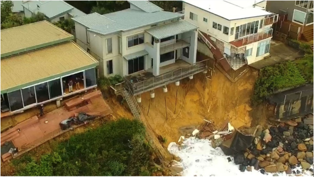
Investigate how rising sea waters might impact a particular coastal town.
Consider the following:
- Australian coastal town to be investigated
- Heights of rising sea levels to be explored
- Local details of the terrain: for example, buildings, cliffs and possible impacts on these.
Exploration
Investigation and analysis of the context or scenario with respect to the questions of interest, conjectures or hypotheses, using mathematical concepts, skills and processes, including the use of technology and application of computational thinking.
- Using the function: f: R → R, f(x) = Af(nx) + c where f is the sine or cosine function, and A,n,c ∈ R with A,n ≠ 0, develop a model that approximates the current tide pattern for the chosen location.
- Revise the approximate tide function developed in step a. to reflect a range of increases in sea level and describe the effect on low and high tides.
- Use interactive predictive and elevation maps to explore the potential effect of different possible sea level rises at your location.
- Consider which other factors might have an impact at the chosen location.
Communication
Summary, presentation and interpretation of the findings from the mathematical investigation and related applications.
Summarise findings and interpret them with respect to the context, stating clearly any assumptions that have been made along the way, and discuss any limitations of the model.
Areas of study
The following content from the areas of study is addressed through this task.
| Unit 2 | |
| Area of study | Content dot point |
| Functions and graphs | 5 |
| Algebra | – |
| Calculus | – |
| Probability and statistics | – |
Outcomes
The following outcomes, key knowledge and key skills are addressed through this task.
| Outcome | Key knowledge dot points | Key skills dot points |
| 1 | 3, 4, 5, | 2, 3, 6 |
| 2 | 1, 5 | 1, 2, 5, 6 |
| 3 | 2, 3, 8 | 6, 11, 13 |
Sample context for assessment: Perimeter and area of a rectangle
Sample context for assessment: Perimeter and area of a rectangle
Introduction
This short task has two parts. The first part is to be completed without technology, and the second part is to be completed with technology.
Part 1
Consider a rectangle with width w and length l.
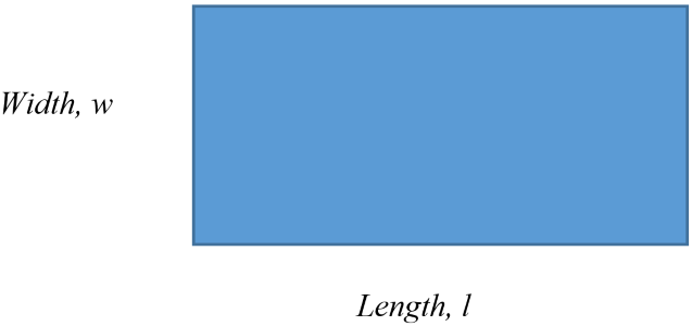
Let the rectangle have a fixed perimeter of 100 cm and vary its area.
- Specify the area of the rectangle as a function of its width and state the domain and range of this function.
- Draw the graph of this function.
- Find the maximum and minimum values for the area of the rectangle and the dimensions for which these occur.
Now let the rectangle have a fixed area of 600 cm2 and vary its perimeter.
- Specify the perimeter of the rectangle as a function of its width and state the domain and range of this function.
- Draw the graph of this function.
- Find the maximum and minimum values for the perimeter of the rectangle and the dimensions for which these occur.
Part 2
The rectangle with width w and length l has a semi-circle with diameter w attached at one end and a half-square triangle with altitude w attached at the other end, forming a composite shape.
Draw and label this composite shape.
Let the shape have a fixed perimeter of 100 cm and vary its area.
- Specify the area of the shape as a function of w and state the domain and range of this function.
- Graph this function.
- Find the maximum and minimum values for the area of the shape and the dimensions for which these occur.
Now let the shape have a fixed area of 600 cm2 and vary its perimeter.
- Specify the perimeter of the shape as a function of w and state the domain and range of this function.
- Graph this function.
- Find the maximum and minimum values for the perimeter of the shape and the dimensions for which these occur.
Areas of study
The following content from the areas of study is addressed through this task.
| Unit 2 | |
| Area of study | Content dot points |
| Functions and graphs | – |
| Algebra | – |
| Calculus | 4, 5 |
| Probability and statistics | – |
Outcomes
The following outcomes, key knowledge and key skills are addressed through this task.
| Unit 2 | ||
| Outcome | Key knowledge dot points | Key skills dot points |
| 1 | 10, 11 | 9, 10 |
| 2 | 1, 2, 5 | 1, 2, 3, 5, 6 |
| 3 | 2, 3, 4 | 3, 5, 6, 7, 9, 12 |
Units 3 and 4
In VCE Mathematical Methods Units 3 and 4, the student's level of achievement will be determined by School-assessed Coursework and two end-of-year examinations. The VCAA will report the student's level of performance as a grade from A+ to E or UG (ungraded) for each of three Graded Assessment components: Unit 3 School-assessed Coursework, Unit 4 School-assessed Coursework and the end-of-year examination.
In Units 3 and 4, school-based assessment provides the VCAA with two judgments:
S (satisfactory) or N (not satisfactory) for each outcome and for the unit; and levels of achievement determined through the specified assessment tasks in relation to all three outcomes for the study. School-assessed Coursework provides teachers with the opportunity to:
- use the designated tasks in the study design
- develop and administer their own assessment program for their students
- monitor the progress and work of their students
- provide important feedback to the student
- gather information about the teaching program.
Teachers should design an assessment task that is representative of the content from the areas of study as applicable, addresses the outcomes and the key knowledge and key skills in accordance with the weightings provided in the study design, and allows students the opportunity to demonstrate the highest level of performance. It is important that students know what is expected of them in an assessment task. This means providing students with advice about relevant content from the areas of study, and the key knowledge and key skills to be assessed in relation to the outcomes. Students should know in advance how and when they are going to be assessed and the conditions under which they will be assessed.
Assessment tasks should be part of the teaching and learning program. For each assessment task students should be provided with the:
- Type of assessment task as listed in the study design and approximate date for completion
- Time allowed for the task
- Nature of the assessment used to measure the level of student achievement
- Nature of any materials they can utilise when completing the task
- Information about the relationship between the task and learning activities, as appropriate.
Following an assessment task:
- Teachers can use the performance of their students to evaluate the teaching and learning program
- A topic may need to be carefully revised prior to the end of the unit to ensure students fully understand content from the areas of study and key knowledge and key skills for the outcomes
- Feedback provides students with important advice about which aspect or aspects of the key knowledge they need to learn and in which key skills they need more practice.
Authentication
- The teacher must consider the authentication strategies relevant for each assessment task. Information regarding VCAA authentication rules can be found in the VCE Administrative Handbook section: Scored assessment: School-based Assessment.
Unit 3 sample assessment tasks
Sample application task: Drug concentrations
Sample application task: Drug concentrations
Introduction
A context such as the following can be used to investigate drug absorption, using a product function model involving circular functions and exponential functions.
For each of the following functions the behaviour and variety of shapes of their graphs is to be investigated. The modelling domain and corresponding range should be identified, as well as key features such as axis intercepts, stationary points and points of inflection, symmetry, asymptotes, and the shape of the graph over its natural domain, using the derivative function for analysis as applicable.
The task will begin with an investigation of a graph that might model the concentration of a certain drug in a patient's system over time. The use of parameters in the family of the function gives students the opportunity to explore the effect the size of parameters has on the graph and hence on the magnitude of the drug in a patient's system over time. Students then explore a similar function that may model the situation more closely.
Component 1
Consider the function with rule f(x) = e-x sin(x).
- Graph the function identifying its key features and explain how the shape of its graph can be deduced from its component functions.
The graph of d(t) = Ae-k tsin(kt), where A and k are positive real constants, can be used to describe drug absorption in a patient's bloodstream, using units mg/litre per unit of time in minutes.
2. Consider the special case where A = 1 and k = 1, and discuss this with respect to a dose of a drug taken at t = 0.
3. Select several pairs of values of A and k where 1 ≤ A ≤ 10 and 0.1 ≤ k ≤ 1, and explore and interpret features of the graph of d(t).
4. Discuss the role of the sine function, the exponential function, and constants A and k where in determining the shape of the graph of d(t).
Component 2
Consider the function d:[0,4π] → R,d(t) = Ae-kt sin(kt), where d(t) measures units mg/l per unit of time in minutes.
- Let A = 10 and k = 0.2. Graph this function, identifying its key features, and construct a corresponding table of values.
- Identify and interpret the maximum rates of increase and decrease, and when the concentration is half of its maximum value.
- Investigate what happens to the graph when A and k are systematically varied, and discuss any patterns.
Jordan is in hospital and needs a particular drug to manage pain.
- Let dj :[0,10] → R,dj (t) = 20e-0.5t sin(0.5t) where the particular drug in Jordan's bloodstream is measured in mg/l and time is measured in minutes. Draw the corresponding graph and compare this with the investigations above.
Component 3
Investigate any points of intersection between graphs of
f:[0,4π] → R,f(t) = Ae-kt sin(kt) and g:[0,4π] → R,g(t) = Ae-kt.
Discuss where these points of intersection exist in relation to the stationary point(s) of the graph of f(t).
Areas of study
The following content from the areas of study is addressed through this task.
| Area of study | Content dot points |
| Functions, relations and graphs | 2, 3, 4, 5, 6 |
| Algebra, number and structure | 4, 5, 6 |
| Calculus | 3, 4, 5 |
| Data analysis, probability and statistics | – |
Outcomes
The following outcomes, key knowledge and key skills are addressed through this task.
| Outcome | Key knowledge dot points | Key skills dot points |
| 1 | 1, 2, 4, 6, 7, 8, 9, 10, 12 | 1, 2, 8, 9, 10, 11, 12 |
| 2 | 1, 2, 3, 5 | 1, 2, 3, 4, 5, 6, 7 |
| 3 | 1, 2, 3, 4, 5, 8 | 1, 2, 3, 4, 5, 6, 7, 9, 10, 11, 12 |
Sample application task: Graphs of products of polynomials
Sample application task: Graphs of products of polynomials
Introduction
A context such as the following could be used to investigate key features of the graphs of some polynomial functions of a real variable formed by products of other polynomial functions.
For each of the following functions the behaviour and variety of shapes of their graphs is to be investigated. The maximal domain and corresponding range should be identified, as well as key features such as axis intercepts, stationary points, points of inflection and symmetry, and the shape of the graph over its natural domain, using the derivative function for analysis as applicable.
The number, location and nature of key features should be determined with respect to different combinations of the parameters that define the product functions, and the different types of graphs identified and classified.
Part 1
Investigate the nature of graphs of polynomial product functions of the form
f:R → R,f(x) = xn (a - x)m
where n and m are positive integers and a ∈ R.
Part 2
Investigate the nature of graphs of polynomial product functions of the form
f:R → R,f(x) = xn (a - x)m
where n and m are positive integers and a ∈ R.
Part 3
Investigate the nature of graphs of polynomial product functions of the form
f:R → R,f(x) = (a - x)n (b - x)m
where n and m are positive integers and a and bare real numbers such that a ≠ b.
Areas of study
The following content from the areas of study is addressed through this task.
| Area of study | Content dot points |
| Functions, relations and graphs | 1, 4, 5 |
| Algebra, number and structure | 1, 2, 5 |
| Calculus | 1, 3, 4, 5 |
| Data analysis, probability and statistics | – |
Outcomes
The following outcomes, key knowledge and key skills are addressed through this task.
| Outcome | Key knowledge dot points | Key skills dot points |
| 1 | 1, 2, 7, 9, 10, 11 | 1, 2, 5, 6, 7, 9, 10, 11, 12 |
| 2 | 1, 2, 3, 5 | 1, 2, 4, 5, 6, 7 |
| 3 | 1, 2, 3, 4, 5, 6, 8 | 1, 2, 3, 4, 5, 6, 7, 9, 11, 12 |
Sample application task: Product functions and pendulum clocks
Sample application task: Product functions and pendulum clocks
The application task is to be of 4–6 hours' duration over a period of 1–2 weeks.
Introduction
A context such as the following could be used to develop an application task that investigates how a product function of an exponential decay function and a circular function can be used to model the motion of the pendulum of a clock after the driving force has stopped.
Component 1
Introduction of the context through specific cases or examples
- Draw the graphs of f:R → R,f(t) = 5e-kt for several (at least five) values of 0 k
- Draw the corresponding graphs of f(-t) and - f(t) on the same set of axes, and comment on the similarities and differences between these graphs.
- Draw the graphs of g:[0,2π] → R,g(x) = sin(ax) for several (at least five) values of a together on the same set of axes. State the period for each function, and comment briefly on the similarities and differences between these graphs.
Component 2
Consideration of general features of the context
- For k = 0.2;a = 1, sketch the graphs of ƒ1(t) = 5e–kt , ƒ2(t) = –5e–kt and s(t) = 5e–kt sin(at), where t ∈ [0, 4π].
- Find the derivative of s(t), in terms of t, k and a, and hence for k = 0.2; a = 1, find the coordinates of the first two maximum/minimum points for s(t) with x coordinates closest to the y-axis.
- Find the coordinates of any points of contact between the graphs of s(t) and ƒ1(t) and between the graphs of s(t) and ƒ2(t). Briefly comment on the relationship between these points of contact and the graph of sin(t). Hence, state the exact x coordinate for the point of intersection closest to the y-axis.
- State the coordinates of intersection between the graphs of s(t) and sin(t), over the given domain. Comment on these findings. Hence, give the exact coordinates of these intersection points.
Component 3
Variation or further specification of assumption or conditions involved in the context to focus on a particular feature or aspect related to the context
Brian has recently purchased a grandfather clock. The rate at which the hands of the clock move is controlled by a pendulum, which is kept in regular motion by slowly descending weighted chains.
When the weights reach their lower point and stop moving, the pendulum swing begins to change, causing the hands of the clock to slow down and gradually stop. From the time when the swing begins to change, the horizontal displacement, s cm, of the point, P, at the end of the pendulum, from the vertical, as shown in the following diagram, can be modelled by functions with the rule
s(t) = 5e–ktsin(at), where t > 0 is the time in seconds after the pendulum swing begins to change and k and a are real constants. For Brian's clock, k = 0.2 and a = 1.
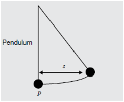
- Find the horizontal displacement of the pendulum for several seconds after the weights stop descending, and draw a series of diagrams corresponding to the position of the pendulum at these times.
- Draw a series of diagrams of the position of the pendulum the first several maxima. If the pendulum is deemed to have come to rest when the swing is less than 0.01 cm, find how long the pendulum takes to come to rest.
- Brian has a friend, Jana, who also bought a similar grandfather clock. Jana's clock is modelled by the same rule for the horizontal displacement when the weights stop descending, where k = 0.4 and a = 1. Draw the graph of the two pendulums' horizontal displacement for t ≥ 22. Compare the behaviour of the two pendulums and discuss how the different values for k affect the motion of the point P after the swing of the pendulum begins to change.
Areas of study
The following content from the areas of study is addressed through this task.
| Area of study | Content dot points |
| Functions, relations and graphs | 2, 3, 4, 5, 6 |
| Algebra, number and structure | 4, 5 |
| Calculus | 2, 3, 4, 5 |
| Data analysis, probability and statistics | – |
Outcomes
The following outcomes, key knowledge and key skills are addressed through this task.
| Outcome | Key knowledge dot points | Key skills dot points |
| 1 | 1, 2, 3,4, 6, 7, 9, 10, 11 | 1, 2, 6, 7, 8, 9, 10, 11, 12 |
| 2 | 1, 2, 5 | 1, 2, 4, 5, 6, 7 |
| 3 | 1, 2, 3, 4, 5, 6, 8 | 1, 2, 3, 4, 5, 6, 7, 9, 11, 12 |
Sample application task: Splining a pathway
Sample application task: Splining a pathway
The application task is to be of 4–6 hours' duration over a period of 1–2 weeks.
Introduction
A context such as the following could be used to develop an application task that investigates how a variety of functions, and piecewise (hybrid) functions constructed from these, could be used to model sections of pathway, such as parts of a bicycle track adjacent to a river, creek or wetland: for example, the Yarra Bend public park in Melbourne.
The process of constructing such a function is called splining.
Component 1
Introduction of the context through specific cases or examples. Students should
Consider the problem of determining a quadratic function f:R → R,f(x) = ax2 + bx + c, the graph of which passes through three specified points. Suppose two of these points, A and B, have coordinates (1, 4) and (2, 2) respectively. The third point, C, has an x-coordinate of 4 and is given as (4, k) where k is an arbitrary real constant.
Explore the effect of varying k on the graph of the function.
- Suppose that C is determined to be (4, 1.5). Investigate cubic functions of the form f:R → R,f(x) = ax3 + bx2 + cx + d with graphs that pass through the points A, B and C.
Explore the effect of d on the behaviour of the graphs of these cubic functions. Identify a value of d that gives a cubic function closely matching the quadratic function that passes through the same three points.
- A fourth point, D, has coordinates (0, m). For different values of m find pairs of quadratic functions, the first pair containing points D, A and B and the second containing the points B and C. These two curves must be smoothly joined at B. Determine the effect of m on the behaviour of the graphs produced.
Component 2
Consideration of general features of the context. Students should
Consider the various sections of the river using different combinations of specified coordinates and dimensions. The following provides a sample.
A new bicycle track is to be constructed along the Yarra River in Kew between two pedestrian bridges labelled A and B on the map shown below.
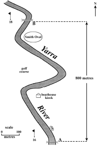
The track cannot be constructed on the western side of the river due to the presence of the golf course.
The track is to follow the curves of the river on the eastern side. That is, it will go from A to B by the boathouse kiosk, passing between the river and Smith Oval.
- Explore how a model can be developed between the pedestrian bridges A and B using a series of smoothly joined quadratic functions.
- Design a measure for how well the pathway matches the curve of the river and apply it to the model.
Component 3
Variation or further specification of assumption or conditions involved in the context to focus on a particular feature or aspect related to the context. Students should
Improve the fit of your bicycle track, according to the measure you have designed, by using a combination of different types of functions.
Alternatively, identify an outline, curve or path in some other context and suitably model this by a piecewise function, which may include function types other than polynomial functions.
Areas of study
The following content from the areas of study is addressed through this task.
| Area of study | Content dot points |
| Functions, relations and graphs | 1, 2, 5, 6 |
| Algebra, number and structure | 1, 4, 5, 6 |
| Calculus | 3, 4 |
| Data analysis, probability and statistics | – |
Outcomes
The following outcomes, key knowledge and key skills are addressed through this task.
| Outcome | Key knowledge dot points | Key skills dot points |
| 1 | 1, 4, 6, 7, 9, 10, | 1, 6, 9, 10, 12 |
| 2 | 1, 2, 3, 5 | 1, 2, 3, 5, 7 |
| 3 | 1, 2, 3, 4, 5, 8 | 1, 2, 3, 4, 5, 6, 7, 9, 11, 12 |
Sample application task: Investigating some polynomial functions
Sample application task: Investigating some polynomial functions
The application task is to be of 4–6 hours' duration over a period of 1–2 weeks.
Introduction
A context such as the following could be used to develop an application task that investigates graphs of polynomial functions of the form f:R → R,f(x) = m(x - a)s(x - b), the key features of these graphs, and the number of solutions to equations of the form
f(x) = p, where p ∈ R.
Component 1
Introduction of the context through specific cases or examples. Students should
- Consider the function f:R → R,f(x) = (x - 1)2 (x - 2). Sketch the graph of y = f(x), and clearly indicate all key features. Find the values of x for which f(x) = p has one, two or three solutions, where p is a real number.
- State the transformations required to map the graph of y = f(x) onto the graph of $y = f\left( \frac{x}{n} \right) + k$ If there is a turning point at (2, 3), find all possible values of n and k. Sketch the corresponding graphs.
- State the transformations required to map the graph of y = f(x) onto the graph of y = Af(x - h). If there is a turning point at
(–1, 4), find all possible values of A and h. Sketch the corresponding graphs.
- The graph of y = f(x) is mapped onto graph of y = Af(n(x - h)) + k. Discuss how the values of A, n, h and k change the graph of the original function under various transformations.
Component 2
Consideration of general features of the context. Students should
- Now consider the function f:R → R, f(x) = m(x - a)2(x - b) where m, a, b ∈ R.
Investigate the graphs of y = f(x) for combinations and ranges of values of the parameters a, b and m.
- In each of the cases in step a., find the values of p ∈ R for which f(x) = p has one, two or three solutions.
- State the transformations required to map the graph of y = f(x) onto the graph of y = Af(nx) + k, where A,n and k ∈ R. Investigate how A,n and k, and a, b and m relate to the location and nature of the stationary points of the graph of
y = Af(nx) + k.
Component 3
Variation or further specification of assumption or conditions involved in the context to focus on a particular feature or aspect related to the context. Students should
- Consider the function f: R → R, f(x) = m(x - a)s (x - b), where m,a,b ∈ R a and s ∈ N. Investigate the graphs of y = f(x) for cases where a 0 and s ∈ N. What generalisations can be made?
- Let f: R → R, f(x) = (x - a)s (x - b) where a,b ∈ R, a and s ∈ N. Find the values of p for which f(x) = p has zero, one, two or three solutions when s = 1, 2, 3, 4 and 5. What generalisations can be made?
Areas of study
The following content from the areas of study is addressed through this task.
| Area of study | Content dot points |
| Functions, relations and graphs | 1, 3, 4, 5 |
| Algebra, number and structure | 1, 4, 5 |
| Calculus | 3, 4, 5 |
| Data analysis, probability and statistics | – |
Outcomes
The following outcomes, key knowledge and key skills are addressed through this task.
| Outcome | Key knowledge dot points | Key skills dot points |
| 1 | 1, 2, 3, 9, 10, 11 | 1, 2, 6, 9, 10, 11, 12 |
| 2 | 1, 2, 3, 5 | 1, 2, 4, 5, 6, 7 |
| 3 | 1, 2, 3, 4, 5, 8 | 1, 2, 3, 4, 5, 6, 7, 9, 11, 12 |
Sample application task: Bezier curves
Sample application task: Bezier curves
The application task is to be of 4–6 hours' duration over a period of 1–2 weeks.
Introduction
A context such as the following could be used to develop an application task that investigates the use of a special kind of cubic polynomial function, called Bernstein polynomials, whose graphs form what are called Bezier curves. These are named after the French automobile engineer Pierre Bezier who developed their application to a new computer-aided design tool for the Renault car manufacturing corporation in the 1960s. Today, Bezier curves are a key component of graphic design applications.
Bezier curves use polynomial functions of low degree, such as cubic polynomials over a restricted domain, to specify the coordinates of the points that make up these curves. These functions, called Bernstein polynomials, provide local control of shape, based on a small set of points called control points, and have graphs that are continuous and smooth curves for which the derivative can be found at any point on the curve. Shapes constructed using drawing packages and the outlines of letters produced by printers are typically based on a set of routines that use these curves.
A cubic Bezier curve drawn over the interval 0 ≤ t ≤ 1 is produced by graphing a relation that has its x and y coordinates specified respectively by the cubic polynomial functions:
x = a(1 - t)3 + 3ct(1 - t)2 + 3et2(1 - t) + gt3
y = b(1 - t)3 + 3dt(1 - t)2 + 3ft2(1 - t) + ht3
Where the coefficients a, b, c, d, e, f, g and h are obtained from the coordinates of the four control points (a, b), (c, d), (e, f) and (g, h).
The gradient of the tangent to the curve for a particular value of t can be determined, using the chain rule for differentiation, by the relationship:
$$\large \frac{dy}{dx} = \frac{dy}{dt} \times \frac{dt}{dx} = \left( \frac{\frac{dy}{dt}}{\frac{dx}{dt}} \right), \quad \frac{dx}{dt} \ne 0$$
The shape of the Bezier curve produced depends on the selection of coordinate values for the control points. Where more than one Bezier curve is used to produce a required shape, these curves will need to be joined smoothly to produce a good image. The three components for an application task could be developed as follows.
Component 1
Introduction of the context: through specific cases or examples students should
- Consider the simpler case of quadratic Bezier curves.
- Select four distinct points as control points and determine the equations for the x and y coordinates as functions of t to specify a particular cubic Bezier curve. Represent the corresponding Bezier curve using a table of values and the graph of the relation.
- Consider the gradient of the tangent to the curve at various points on the curve, including the relation between the tangents to the first and last control points and the location of the second and third control points.
Component 2
Consideration of general features of the context students should
- Vary the control points and consider the Bezier curves produced, including cases that lead to, for example, straight lines and loops.
- Investigate the selection of control points to produce a reasonable representation of a particular shape: for example, how many letters of the alphabet can be reasonably approximated by a single Bezier curve?
- Consider how well a cubic Bezier curve matches the required shape and any limitations on possible shapes that can be represented using these curves.
Component 3
Variation or further specification of assumption or conditions involved in the context to focus on a particular feature or aspect related to the context. Students should
- Represent more complicated shapes formed by piecing together several Bezier curves.
- Identify the location of control points for a pair of cubic Bezier curves that are smoothly joined to represent other letters, or for several Bezier curves that are smoothly joined to represent a shape such as the outline or cross section of a car.
Areas of study
The following content from the areas of study is addressed through this task.
| Area of study | Content dot points |
| Functions, relations and graphs | 1, 5, 6 |
| Algebra, number and structure | 1, 5 |
| Calculus | 3, 4 |
| Data analysis, probability and statistics | – |
Outcomes
The following outcomes, key knowledge and key skills are addressed through this task.
| Outcome | Key knowledge dot points | Key skills dot points |
| 1 | 1, 3, 4, 7, 10, 11 | 1, 2, 7, 9, 11, 12, 13 |
| 2 | 1, 2, 3, 5 | 1, 2, 3, 4, 6, 7 |
| 3 | 1, 2, 3, 4, 5, 8 | 1, 2, 3, 4, 5, 6, 7, 9, 11, 12 |
Unit 4 sample assessment tasks
Sample Modelling or problem-solving task: Proportions of popularity
Sample Modelling or problem-solving task: Proportions of popularity
The modelling or problem-solving task is to be of 2–3 hours' duration over a period of 1 week.
Introduction
Polls provide a topical and regular insight into the relative popularity of political parties over time, in particular as events occur and are reported in the media and trends change.
Popularity on a two-party preferred basis as indicated by polls is a context for inference about proportions with respect to a population based on sampling. Consider a country that has a population of around 15 million voters on an electoral roll. Polls inform public consideration and debate on various matters of policy.
Part 1
- Plot graphs of the distribution of sample proportions for sample sizes of 50, 100 and 200 for
p = 0.43, 0.52, 0.61
2. Explain what these graphs indicate.
Part 2
- Randomly select an integer in the range [30, 60] and use this to generate a population of 1000 voters, with that value as the percentage of the population who would vote for a given party on a two-party preferred basis.
- Generate 50 random samples of size n = 60 from this population and use each of these to find a point estimate for the true population proportion. Graph the distribution of the sample proportions and state its mean and standard deviation.
- Use each point estimate to construct a confidence interval for p at a 90% level of confidence. Graph all of these intervals together as a set of horizontal line segments, one under the other, and use them to explain the relationship between the true value of the population proportion, p, and this set of confidence intervals for a 90% level of confidence.
Part 3
The Margin of Error Table relates sample size, sample proportion and margin of error at a 95% level of confidence.
- Show how the figures for the row corresponding to a sample size of 2000 are obtained.
- Draw graphs of several functions to illustrate how the maximum margin of error varies for different sample sizes and levels of confidence.
- Suppose that it costs $50 per individual response gathered as part of a survey. Discuss what you think might be a reasonable combination of sample size, level of confidence, margin of error and total cost.
Areas of study
The following content from the areas of study is addressed through this task.
| Area of study | Content dot points |
| Functions, relation and graphs | – |
| Algebra, number and structure | – |
| Calculus | – |
| Data analysis, probability and statistics | 1, 2, 4 |
Outcomes
The following outcomes, key knowledge and key skills are addressed through this task.
| Outcome | Key knowledge dot points | Key skills dot points |
| 1 | 1, 14, 16, 17 | 1, 16, 18, 19, 20 |
| 2 | 1, 2, 4, 5 | 1, 2, 3, 4, 6, 7 |
| 3 | 1, 2, 3, 4, 6, 7, 8 | 1, 3, 4, 5, 8, 9, 10, 11 |
Sample Modelling or problem-solving task: Close to normal
Sample Modelling or problem-solving task: Close to normal
The modelling or problem-solving task is to be of 2–3 hours' duration over a period of 1 week.
Introduction
A context such as the following could be used to develop a two-part problem-solving task that involves a composition of functions leading to the standard normal distribution, and the use of simulations to investigate the distribution of proportions in probability experiments.
Part 1
Let f: R → R,f(x) = ex and g: R → R,g(x) = -x2.
- Plot the graphs of f(x) and g(x) and explain how the shape of the graph of f(g(x)) can be deduced from these.
- Plot the graph of f(g(x)) and clearly identify its key features.
- Use sets of trapeziums to form a sequence of under-estimates and over-estimates for the area bounded by the graph of f(g(x)) and the horizontal axis between x = –10 and x = 10.
- Use the results from step c. to find approximate values for a and b such that h: R → R,h(x) = ae-bx2 forms a probability density function, with mean 0 and standard deviation 1.
- Plot the graph from step d. on the same set of axes as the standard normal distribution and comment on similarities and differences.
Part 2
- A pair of standard dice are rolled simultaneously. Use technology to simulate this experiment for 60 rolls of the dice and record the set of outcomes. What is the proportion of rolls for which the two dice had the same value?
- Run the simulation 100 times and plot the distribution of this proportion. Describe the distribution.
- Now consider two identical packs of 10 cards numbered 1 to 10. Both packs are shuffled thoroughly. The first card is turned over from each pack and the result is recorded. This is then repeated for the second card from each pack, the third card from each pack and so on, through to the 10th and final card of each pack. Use technology to simulate this experiment and record the set of outcomes. How many pairs of cards in the experiment had the same value?
- Run this simulation 100 times and plot the distribution of proportions for the number of times when the pair of cards had the same value. Describe this distribution.
- Give an estimate for the probability that there is at least one pair of matching cards and explain how this estimate was obtained.
Areas of study
The following content from the areas of study is addressed through this task.
| Area of study | Content dot points |
| Functions, relations and graphs | 2, 3, 4, 5 |
| Algebra, number and structure | 3, 5 |
| Calculus | 3, 4, 7, 9 |
| Data analysis, probability and statistics | 1, 2, 3 |
Outcomes
The following outcomes, key knowledge and key skills are addressed through this task.
| Outcome | Key knowledge dot points | Key skills dot points |
| 1 | 1, 2, 4, 6, 7, 11, 12, 13, 14, 17 | 1, 2, 4, 5, 12, 14, 15, 16, 17, 18, 19, 20 |
| 2 | 1, 2, 4, 5 | 1, 2, 3, 4, 5, 6, 7 |
| 3 | 1, 2, 3, 4, 7, 8 | 1, 2, 3, 4, 5, 6, 8, 9, 10, 11, 12, 13 |
Sample Modelling or problem-solving task: Traversing terrains
Sample Modelling or problem-solving task: Traversing terrains
The modelling or problem-solving task is to be of 2–3 hours' duration over a period of 1 week.
Introduction
A context such as the following could be used to develop a modelling or problem-solving task that involves modelling travel over different terrains at different average speeds for each terrain, and using this information to optimise the time of travel. Bushwalkers travel over different types of terrain, from cleared to dense bush. The denseness of the bush and the ruggedness of the terrain influence the average speed of travel. By planning a route to take such factors into consideration, the total time taken to travel from one point to another can be optimised. In calculating estimates of the time for a particular route, a walker uses his or her average speed for each different type of terrain they are likely to encounter.
For a walk through a particular type of terrain, the distance travelled, d km, can be calculated as the product of the average speed, v km/h, and the time travelled at this speed, t hours. On a typical two-day walk a bushwalker might cover a distance of up to 30 km with walking speeds of up to 5 km/h over cleared terrain.
Part 1
- For a typical two-day walk, choose several representative values for average speed and draw a graph of the relationship between t and d for each of these values.
- Similarly, choose several representative values for the distance to be travelled and draw a graph of the relationship between t and v for each of these values.
- Discuss the key features of each of the two families of graphs and the differences between them.
Part 2
A bushwalk is planned from Ardale to Brushwood. As shown in the diagram below.
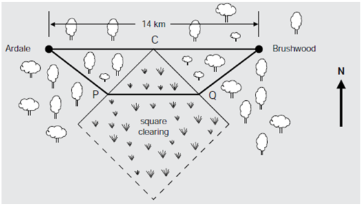
The direct route, a distance of 14 km, goes entirely through rugged bush country. However, there is a large square clearing situated as shown. This clearing has one diagonal along the perpendicular bisector of the direct route and one corner, C, at the midpoint of the direct route.
One of the bushwalkers believes that time will be saved if they travel from Ardale to Brushwood on a route similar to the one shown passing through P and Q, where the section PQ is parallel to the direct route. The side length of the square clearing is 7 km, and the part of this route that goes across the square clearing is parallel to the direct route.
- Choose a suitable variable, and hence determine a mathematical relationship that can be used to determine the total time for a route of this type. Draw the graph of this relationship and discuss its key features.
- Find and describe the route for which the travelling time will be least and compare it with the direct route.
Areas of study
The following content from the areas of study is addressed through this task.
| Area of study | Content dot point(s) |
| Functions, relations and graphs | 6 |
| Algebra, number and structure | 5 |
| Calculus | 1, 4, 5 |
| Data analysis, probability and statistics | – |
Outcomes
The following outcomes, key knowledge and key skills are addressed through this task.
| Outcome | Key knowledge dot points | Key skills dot points |
| 1 | 1, 4, 6, 7, 9, 10 | 1, 6, 9, 12 |
| 2 | 1, 2, 3, 5 | 1, 2, 3, 4, 5, 6, 7 |
| 3 | 1, 2, 3, 4, 5, 6, 8 | 1, 2, 3, 4, 5, 6, 7, 9, 10, 11, 12, 13 |
Sample modelling or problem-solving task – wall and window
Sample modelling or problem-solving task – wall and window
The modelling or problem-solving task is to be of 2 - 3 hours duration over a period of 1 week.
Introduction
A context such as the following could be used to develop a modelling or problem-solving task which involves modelling the shape of a designer two-part window feature for a section of wall, and the dimensions and area of the design.
The section of the wall is 4 m wide and 3.5 m high. The window is a symmetrical design which fits in the middle of the wall horizontally. The base of the window forms a straight line 0.5 m above and parallel to the floor and is 2 m in length. The lower part of the window has two straight line slant edges, and these are 1.5 m apart at the height of 1.5 m from the floor. The window designer is considering a range of possibilities for the upper part of the window, the highest point of which is to be at most 3 m from the floor.
The designer constructs a graph of the window design using a set of axes with the origin on the floor at the middle of the wall.
Part 1
Initially the designer considers and upper part consisting of two-line segments which join onto the top of the lower straight edges, at an angle of 45° to the horizontal, and extend to the point where they meet.
- Use functions to define the sections of the window's edges and draw a graph showing the wall and the window, labelling all key points with their coordinates.
- Find the area of the window.
- Consider a family of related designs where the angle the edges of the upper part make with the horizontal is varied. Show several examples and calculate the area of the window in each case. What is the largest possible value for this angle, and the corresponding area of the window?
Part 2
As an alternative, the designer considers using an arch for the top part of the window.
- Draw the graph where the arch is a semi-circle. Calculate the area of the window. Do the lower and upper parts of the window join smoothly?
- Draw several graphs for the upper part defined by the family of functions with rule of the form f(x) = ax2 + b, where a and b are non-zero real constants.
- For the case where the lower and upper parts of the window join smoothly, calculate the corresponding area of the window.
- What happens when a function with rule of the form g(x) = a sin(bx) + c is used to model the upper arch, if the two parts are to be smoothly joined?
Part 3
The designer decides that while a smooth join of the two parts of the window is a critical requirement, it is not necessary for the arch to be smooth at its top point, so a symmetrical hybrid function based on part of the graph of some other function could be used to represent the arc.
Consider some other possible modelling functions and identify which of these gives the maximum window area for different choices of functions and defining parameters.
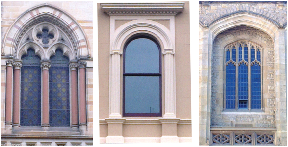
The following images show some arches from buildings along North Terrace in Adelaide.
Areas of study
The following content from the areas of study is addressed through this task.
| Area of study | Content dot point |
| Functions, relations and graphs | 2, 3, 6 |
| Algebra, number and structure | 5, 6, |
| Calculus | 3, 4, 5, 6, 10 |
| Data analysis, probability and statistics | - |
Outcomes
The following outcomes, key knowledge and key skills are addressed through this task.
| Outcome | Key knowledge dot point | Key skill dot point |
| 1 | 1, 2, 4, 7, 10, 12 | 1, 2, 6, 10, 12, 13, 14, 15 |
| 2 | 1, 2, 3, 5 | 1, 2, 3, 5, 7 |
| 3 | 2, 3, 4, 5, 8 | 2, 3, 4, 5, 6, 7, 9, 11, 12, 13 |
School-assessed Coursework videos
A series of videos and materials to help teachers develop School-assessed Coursework.
Performance descriptors
The VCAA performance descriptors are advice only and provide a guide to developing an assessment tool when assessing the outcomes of each area of study. The performance descriptors can be adapted and customised by teachers in consideration of their context and cohort, and to complement existing assessment procedures in line with the VCE Administrative Handbook and the VCE assessment principles.
Application task performance criteria
Unit 3, Outcome 1
Unit 3 | Mark range | Criterion |
| 0–3 | Appropriate use of mathematical conventions, symbols and terminology Application of mathematical conventions in diagrams, tables, and graphs, such as axes labels and conventions for asymptotes. Appropriate and accurate use of symbolic notation in defining mathematical terms or expressions, such as formulas, equations, transformations and combinations of functions. Use of correct expressions in symbolic manipulation or computation in mathematical work. Use of correct terminology, including set notation, to specify relations and functions, such as domain, co-domain, range, and rule. Description of key features of relations and functions as applicable, such as symmetry, periodicity, asymptotes, coordinates for axial intercepts, stationary points and points of inflection. | |
| 0–6 | Definition and explanation of key concepts Definition of mathematical concepts using appropriate terminology, phrases, and symbolic expressions. Provision of examples which illustrate key concepts and explain their role in the development of related mathematics. Statement of conditions or restrictions which apply to the definition of a concept. Identification of key concepts in relation to each area of study and explanation of the use of these concepts in applying mathematics in different practical or theoretical contexts. | |
| 0–6 | Accurate use of mathematical skills and techniques Use of algebra and numerical values to evaluate expressions, substitute into formulas, construct lists and tables, produce graphs and solve equations. Use of mathematical algorithms, routines and procedures involving algebra, functions, coordinate geometry, calculus to obtain results and solve problems. Identification of domain and range of a function or relation and other key features using numerical, graphical, and algebraic techniques, including approximate or exact specification of values. | |
| Outcome 1 mark allocation | 15 marks | |
Unit 3, Outcome 2
Unit 3 | Mark range | Criterion |
| 0–4 | Identification of important information, variables and constraints Identification of key characteristics of a problem, task or issue and statement of any assumptions underlying the use of relevant mathematics in the given context. Choice of suitable variables, parameters, and constants for the development of mathematics related to various aspects of a given context. Specifications of constraints, such as domain and range constraints, and relationships between variables, related to aspects of a context. | |
| 0–8 | Application of mathematical ideas and content from the specified areas of study Demonstration of understanding of key mathematical content from one or more areas of study in relation to a given context. Use of specific and general formulations of concepts and mathematical content drawn from the areas of study to derive results for analysis in this context. Key elements of algorithm design including sequencing, decision-making and repetition, and their representation and implementation. Appropriate use of examples to illustrate the application of a mathematical process, or use of a counter-example to disprove a proposition or conjecture. Use of a variety of approaches to develop functions as models for data presented in tabular, diagrammatic, or graphical form. Use of algebra, coordinate geometry, derivatives, gradients, anti-derivatives, and integrals, to set up and solve problems. | |
| 0–8 | Analysis and interpretation of results Analysis and interpretation of results obtained from examples or counter-examples to establish or refute general case propositions or conjectures related to a context for investigation. Generation of inferences from analysis to draw conclusions related to the context for investigation, and to verify or modify conjectures. Discussion of the validity and limitations of any models. | |
| Outcome 2 mark allocation | 20 marks | |
Unit 3, Outcome 3
Unit 3 | Mark range | Criterion |
| 0–6 | Appropriate selection and effective use of technology Relevant and appropriate selection and use of technology, or a functionality of the selected technology for the mathematical context being considered. Distinction between exact and approximate results produced by technology, and interpretation of these results to a required accuracy. Use of appropriate range and domain and other specifications which illustrate key features of the mathematics under consideration. | |
| 0–9 | Application of technology Analysis of the relationship of the results from an application of technology to the nature of a particular mathematical question, problem, or task. Use of tables of values, families of graphs or collections of other results produced using technology to support analysis in problem-solving, investigative, or modelling contexts. Production of results efficiently and systematically which identify examples or counter-examples which are clearly relevant to the task. Use of computational thinking, algorithms, models and simulations to solve problems related to a context. | |
| Outcome 3 mark allocation | 15 marks | |
A sample record sheet for the application task can be used to record student level of achievement with respect to the available marks for the performance criteria relating to each outcome, and to indicate pointers corresponding to relevant aspects of the task.
Modelling or problem-solving task performance criteria
Unit 4, Outcome 1
Unit 4 | Mark range | Criterion |
| Task 1 0–2 | Appropriate use of mathematical conventions, symbols and terminology Application of mathematical conventions in diagrams, tables, and graphs, such as axes labels and conventions for asymptotes. Appropriate and accurate use of symbolic notation in defining mathematical terms or expressions, such as equations, transformations and combinations of functions. Use of correct expressions in symbolic manipulation or computation in mathematical work. Use of correct terminology, including set notation, to specify relations and functions, such as domain, co-domain, range and rule. Description of key features of relations and functions, including probability mass and density functions as applicable, such as symmetry, periodicity, asymptotes, coordinates for axial intercepts, stationary points and points of inflection. | |
| Task 2 0–2 | ||
| Task 1 0–3 | Definition and explanation of key concepts Definition of mathematical concepts using appropriate terminology, phrases, and symbolic expressions. Provision of examples which illustrate key concepts and explain their role in the development of related mathematics. Statement of conditions or restrictions which apply to the definition of a concept. Identification of key concepts in relation to each area of study and explanation of the use of these concepts in applying mathematics in different practical or theoretical contexts. | |
| Task 2 0–2 | ||
| Task 1 0–3 | Accurate use of mathematical skills and techniques Use of algebra and numerical values to evaluate expressions, substitute into formulas, construct tables, produce graphs and solve equations. Use of mathematical routines and procedures involving algebra, functions, coordinate geometry, calculus, probability, and statistics to obtain results and solve problems. Identification of domain and range of a function or relation and other key features using numerical, graphical and algebraic techniques, including approximate or exact specification of values. Identification and representation of sample spaces. | |
| Task 2 0–3 | ||
| Outcome 1 mark allocation | 15 marks | |
Unit 4, Outcome 2
Unit 4 | Mark range | Criterion |
| Task 1 0–2 | Identification of important information, variables and constraints Identification of key characteristics of a problem, task or issue and statement of any assumptions underlying the use of relevant mathematics in the given context. Choice of suitable variables, including random variables, parameters, and constants for the development of mathematics related to various aspects of a given context. Specifications of constraints, such as domain and range constraints, and relationships between variables, related to aspects of a context. | |
| Task 2 0–2 | ||
| Task 1 0–4 | Application of mathematical ideas and content from the specified areas of study Demonstration of understanding of key mathematical content from one or more areas of study in relation to a given context. Use of specific and general formulations of concepts and mathematical content drawn from the areas of study to derive results for analysis in this context. Key elements of algorithm design including sequencing, decision-making and repetition, and their representation and implementation. Appropriate use of examples to illustrate the application of a mathematical process, or use of a counter-example to disprove a proposition or conjecture. Use of a variety of approaches to develop functions as models for data or distributions presented in tabular, diagrammatic, or graphical form. Use of algebra, coordinate geometry, derivatives, gradients, anti-derivatives, and integrals, to set up and solve problems. | |
| Task 2 0–4 | ||
| Task 1 0–4 | Analysis and interpretation of results Analysis and interpretation of results obtained from examples or counter-examples to establish or refute general case propositions or conjectures related to a context for investigation. Generation of inferences from analysis to draw conclusions related to the context for investigation, and to verify or modify conjectures. Discussion of the validity and limitations of any models. | |
| Task 2 0–4 | ||
| Outcome 2 mark allocation | 20 marks | |
Unit 4, Outcome 3
Unit 4 | Mark range | Criterion |
| Task 1 0–3 | Appropriate selection and effective use of technology Relevant and appropriate selection and use of technology, or a function of the selected technology for the mathematical context being considered. Distinction between exact and approximate results produced by technology, and interpretation of these results to a required accuracy. Use of appropriate range and domain and other specifications which illustrate key features of the mathematics under consideration. | |
| Task 2 0–3 | ||
| Task 1 0–4 | Application of technology Use and interpretation of the relation between numerical, graphical, and symbolic forms of information produced by technology about functions, equations and distributions, and their corresponding features. Analysis of the relationship of the results from an application of technology to the nature of a particular mathematical question, problem or task. Use of tables of values, families of graphs or collections of other results produced using technology to support analysis in problem solving, investigative or modelling contexts. Production of results efficiently and systematically which identify key features, examples or counter-examples which are clearly relevant to the task. Use of computational thinking, algorithms, models and simulations to solve problems related to a context. | |
| Task 2 0–5 | ||
| Outcome 3 mark allocation | 15 marks | |
A sample record sheet for modelling or problem-solving task 1 and a sample record sheets for modelling or problem-solving task 2 can be used to record student level of achievement with respect to the available marks for the performance criteria relating to each outcome, and to indicate pointers corresponding to relevant aspects of the task.
- Sample record sheet for the application task
- Sample record sheet for modelling or problem-solving task 1
- Sample record sheet for modelling or problem-solving task 2
These performance criteria can be used in several ways:
- directly in conjunction with the sample record sheets and teacher annotations for pointers with respect to key aspects of the task related to each criterion for the outcomes
- directly with the descriptive text for each criterion modified to incorporate task specific elements as applicable
- as a template for teachers to develop their own criteria and descriptive text for each criterion, including their own allocation of marks for the criteria with the total mark allocation for each outcome as specified in the study design, using their own record sheets.