Teaching and Learning
Accreditation period Units 1-4 from 2023
Learning activities
Each of the following learning activities is linked to the sample course plan. They illustrate some of the ways in which aspects of mathematics learning can be addressed, and include a cross reference to content from the areas of study and key knowledge and key skills for the outcomes.
Unit 1
Learning activity: Lines and Graphs
Learning activity: Lines and Graphs
Introduction
This learning activity explores properties of line segment graphs and their application.
Part 1
Consider the set of points and coordinates given below:
| Point | A | B | C | D | E | F |
| Coordinates | (0,0) | (5,3) | (7,10) | (15,10) | (17,2) | (17,0) |
- Plot these points on a cartesian set of axes, and connect them to form the line segments AB, BC, CD, DE and EF.
- Find the slope of each line segment.
- Find the equation of the line that contains each line segment.
Part 2
- Use technology to draw the corresponding line segment graph.
- State the values that each variable may take.
Part 3
- Define a rule that models the Australian income tax scales and draw the corresponding line segment graph for incomes up to \$250,000.
- Construct a table of values that shows the tax payable for incomes up to \$250,000 in steps of \$10,000.
- Compare with the corresponding tax rule for the US.
Areas of study
The following content from the areas of study is addressed through this learning activity.
Area of study | Topic | Content dot point |
| Functions, relations and graphs | Linear functions, graphs, equations and models | 1, 2, 4 |
Outcomes
The following outcomes, key knowledge and key skills are addressed through this task.
Outcome | Key knowledge dot point | Key skill dot point |
| 1 | 1, 2, 3, 4 | 1, 2, 3, 5 |
| 2 | 1, 2, 3, 4 | 1, 2, 3, 4 |
| 3 | 3, 4, 5 | 3, 4, 5, 6, 7, 9, 11, 12 |
Learning activity: Matrices
Learning activity: Matrices
Introduction
This learning activity explores how pairs of people in a network can communicate with each other.
Part 1
Consider four employees in a company. Because of their positions and level of power within the company, not every level of employment communicates with the other.
For example:
- The CEO (Charles) speaks to the General Manager (Greta) about financial planning.
- The Assistant Manager (Abbey) speaks to the General Manager about protocol.
- The clerk (Ken) speaks to the General Manager to ask if he wants any jobs done.
- The General Manager on any given workday will talk to the CEO, the Assistant Manager and the clerk.
The information could be represented by a diagram called a social network.
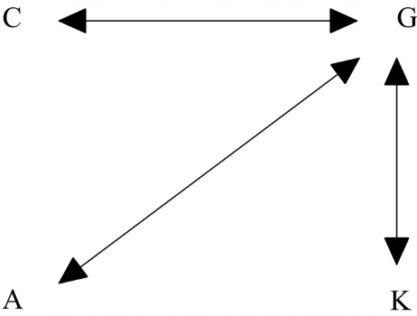
We can see that, for example, the CEO does not communicate directly with the Assistant Manager on any given workday, but communicates with the General Manager. This is called a one-step communication link.
We assume communication is a two-way process. So, if C communicates with G, then G communicates with C.
We can form a 4 × 4 matrix to represent the one-step communications.
In the matrix C representing the connections, we use a 1 to indicate that two people directly communicate and 0 if they do not.
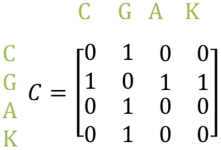
- What information is given by the element ${\large C_{13}}$?
- What information is given by the element ${\large C_{24}}$?
- What information is given by the sum of column G?
Part 2
Two-step communication
The CEO can communicate with the Assistant Manager by sending a message via the General Manager, who we can see speaks to both of them. This is called a two-step communication link.
While we can use a diagram to work out the one-step and two-step communication links, it is convenient to show the two-step links and the total of one-step and two-step links in matrices.
The matrix ${\large C^{2}}$ gives the number of two-step communications between the workers.
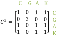
So, if we look at the first column, we can see that Charles can talk to Abbey and Ken via one other person (Greta).
There is also a 1 for element ${\large C^{2}_{11}}$. Initially this may not appear very meaningful that Charles can talk to himself; however, it could be interpreted that the two-step communication link for Charles back to himself represents (for example) him asking one other person (Greta) to remind him of something at a future time.
- What information is given by the element ${\large C^{2}_{43}}$?
- What information is given by the element ${\large C^{2}_{32}}$?
- Why is there a 3 for element ${\large C^{2}_{22}}$?
Part 3
It may also be useful to determine the total, T, of the one and two step links in a communication matrix system.
For this example,
${\large T = C + C^2}$
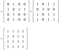
There are no 0 elements in the matrix. What does this indicate?
Areas of study
The following content from the areas of study is addressed through this learning activity.
Area of study | Topic | Content dot point |
| Discrete mathematics | Matrices | 1, 3, 4 |
Outcomes
The following outcomes, key knowledge and key skills are addressed through this task.
| Outcome | Key knowledge dot point | Key skill dot point |
| 1 | 1, 3, 5 | 3, 4 |
| 2 | 1, 2, 3 | 1, 2, 3, 4 |
| 3 | 1, 4, 5 | 3, 4, 5, 7, 10, 12 |
Learning activity: Percentages and applications
Learning activity: Percentages and applications
Introduction
This learning activity explores percentages in relation to financial applications and GST.
Part 1
Percentage increase
If a value P increases by r % write an expression for its new value.
a. A \$70 shirt is marked up by 15%. What is its new price?
Percentage decrease
If a value P decreases by r % write an expression for its new value.
b. A \$23 book is discounted by 20%. What is its sale price?
Percentage change
Write a rule to calculate the percentage change given the original price of an item.
c. The price of a hat was increased from \$40 to \$50. What percentage increase was applied?
d. The price of a T-shirt was reduced from \$40 to \$32. What was the percentage discount applied?
Calculating original price
Write rules to calculate the original price given the marked up or discounted price of an item.
e. The sale price of a jacket is \$102. If the jacket has been discounted by 15%, what was the original price of the jacket?
Part 2
Goods and services tax (GST)
The goods and services tax (GST) is a tax of 10% that is added to the price of most goods (e.g. cars) and services (e.g. insurance).
Write a rule that will calculate the cost with GST applied, considering a factor by which the cost without GST must be multiplied. How can this conversion factor be used to calculate the cost without GST from a cost with GST applied?
a. If the cost of electricity supplied in one month is \$288.50, how much will the customer be charged once GST is added to the bill?
- Write a rule to calculate the cost without GST from the cost inclusive of GST.
b. A customer was charged \$33, GST included, for a new belt. What was the cost of the belt before GST was added?
- Write a rule for the amount of GST to be added to the original cost of goods and services.
c. If the cost of electricity supplied in one month is \$288.50, how much GST is added to the bill?
- Write a rule for the amount of GST that was added given the cost inclusive of GST.
d. A customer was charged \$33, GST included, for a new belt. How much GST was added to the price of the belt.
Areas of study
The following content from the areas of study is addressed through this learning activity.
Area of study | Topic | Content dot point |
| Algebra, number and structure | Financial mathematics | 8, 9 |
Outcomes
The following outcomes, key knowledge and key skills are addressed through this task.
Outcome | Key knowledge dot point | Key skill dot point |
| 1 | 6 | 2 |
| 2 | 1, 2, 3 | 1, 2, 3, 4 |
| 3 | 1, 4, 5 | 3, 4, 5, 7, 10, 12 |
Unit 2
Learning activity: Rail networks and types of graphs
Learning activity: Rail networks and types of graphs
Introduction
The rail network in any large city is structured and complex.
Research a rail network in one of the Australian Capital cities. Also research proposed changes to this city's rail network that will take place in the next 10 years.
Part 1
- Choose 10 rail stations from at least three different lines in your chosen city.
- Construct a network involving these 10 stations using vertices and edges and current or planned connections that exist between each station.
- Describe the network constructed using the language and type of graph.
- Choose two stations from the constructed network and from different lines. Display and describe the current walk that would be needed to travel between these stations. Include how this journey could be made more efficient.
- Discuss and justify the number of edges that would need to be included to enable efficient travel between two selected stations. Also include a discussion on the benefits and limitations linked to cost, economy and infrastructure.
Part 2
- Using a detailed map include distances between stations on a network of the 10 selected stations taken from at least three separate lines.
- If a communication cable was included in the network, investigate where it would be added to ensure the shortest amount of cable was used.
- Calculate the distance needed to travel to every station. Investigate how this distance could be minimised by the addition of other connections between stations. Discuss the cost that would be linked to the additional connections, the total length of the additional connections and if this would be a viable option.
Areas of study
The following content from the areas of study is addressed through this learning activity.
Area of study | Topic | Content dot point |
| Discrete mathematics | Graph and networks | 1, 3, 4, 5 |
Outcomes
The following outcomes, key knowledge and key skills are addressed through this task.
Outcome | Key knowledge dot point | Key skill dot point |
| 1 | 1, 2, 3 | 2, 3, 4, 5 |
| 2 | 1, 2, 3, 4 | 1, 2, 3, 4 |
| 3 | 1, 2, 5 | 1, 2, 8, 10, 11 |
Learning activity: Planning a house and land package
Learning activity: Planning a house and land package
Introduction
A design for a house and land package is requested. There is flexibility in a number of aspects of this design that can be explored.
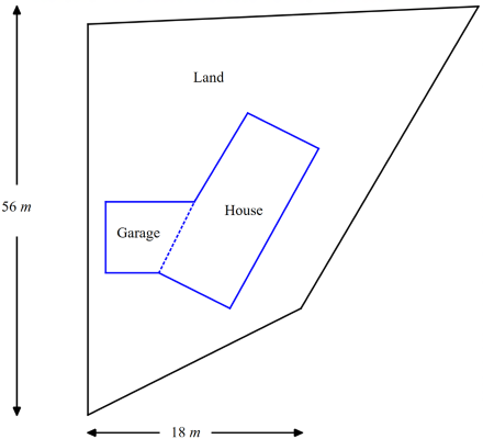
The restrictions on the design are:
- The land is 1800 m2 in size.
- The size of the house and garage must be between 180 – 220 m2.
- The house is built as a rectangle and the garage is built as a trapezium.
- The garage and house must be built so there is at least 1.5 m between any wall and the land boundary.
- The land shape cannot have any right angles.
Formulation
Investigate the shape and size of the house, garage and land in order for these constraints to be met. If certain constraints cannot be met, suggest an alternative and explain your reasoning.
Communication
Construct a scaled image of the design including all relevant measurements (lengths, angles, areas) and present you findings in a concise report.
Areas of study
The following content from the areas of study is addressed through this learning activity.
Area of study | Topic | Content dot point |
| Space and measurement | Space, measurement and applications of trigonometry | 1, 2, 3, 4, 7, 8 |
Outcomes
The following outcomes, key knowledge and key skills are addressed through this task.
Outcome | Key knowledge dot point | Key skill dot point |
| 1 | 1, 4, 5, 7, 8 | 2, 5, 6, 7 |
| 2 | 1, 2, 3, 4 | 1, 2, 3, 4 |
| 3 | 1, 2, 4, 5 | 1, 2, 3, 7, 8, 9, 10, 11, 12 |
Learning activity: Variation in random samples
Learning activity: Variation in random samples
Introduction
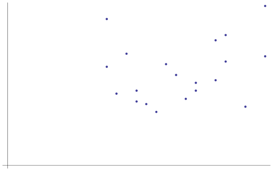
The task uses different sets of random data to create scatterplots and the associated equations of the lines of good fit by eye are analysed for their similarities and differences.
This activity could be carried out with the use of the relevant technology for constructing and printing scatterplots so that a line of good fit by eye can be drawn.
Part 1
- i. Randomly generate a set of 20 ordered pairs with integer coordinates from within a given interval of x-values and a given interval of y-values. ii. Draw a scatterplot of the corresponding points. Add a line of good fit by eye and calculate the equation of this line.
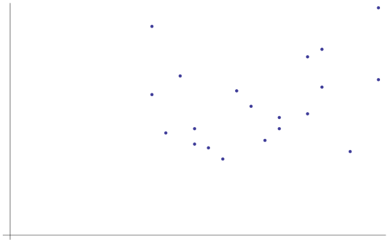
- Repeat the above random generation of 20 ordered pairs, construct the linked scatterplot and calculate the equation of the line of good fit by eye.
- Discuss the similarities and differences between the calculated equations of the lines of good fit by eye.
Part 2
- i. Expand the given interval to choose the required integer values. Randomly generate a set of 20 ordered pairs (x - and y -values) with integer coordinates from this adjusted interval of x- and y -values. ii. Draw a scatterplot of the corresponding points. Add a line of good fit by eye and calculate the equation of this line.
- Repeat the above random generation of 20 ordered pairs, construct the linked scatterplot and calculate the equation of the line of good fit by eye.
- Discuss the similarities and differences between the calculated equations of the lines of good fit by eye found in Part 2 compared to those found in Part 1.
Part 3
Increase the sample size of ordered pairs to investigate.
Discuss the impact of an increased sample size on the equations of good fit found by eye calculated in Part 3, as compared to previous parts.
Areas of study
The following content from the areas of study is addressed through this learning activity.
| Area of study | Topic | Content dot point |
| Data analysis, probability and statistics | Investigating relationships between two numerical variables | 2, 3, 4, 5 |
Outcomes
The following outcomes, key knowledge and key skills are addressed through this task.
| Outcome | Key knowledge dot point | Key skill dot point |
| 1 | 2, 3, 4 | 1, 2, 3, 4 |
| 2 | 1, 2, 4 | 1, 3, 4 |
| 3 | 1, 3, 4, 5 | 1, 3, 4, 5, 6, 7, 8, 9, 10, 11, 12 |
Learning activity: Variation and correlation
Learning activity: Variation and correlation
Introduction
The task involves varying the location of some points on a scatterplot and observing corresponding changes in the value of r, the Pearson correlation coefficient.
This activity should be carried out with the use of the relevant technology for constructing scatterplots and calculating correlation coefficients and the equations of regression lines.
Part 1
Construct a set of 20 ordered pairs with integer coordinates randomly selected from within a given interval of x-values and a given interval of y-values.
- Draw a scatterplot of the corresponding points, calculate the correlation, and find the equation of the corresponding regression line. Plot this line on the same set of axes.
- Vary the location of some points to produce a close to 0.5 correlation, find the equation of the corresponding regression line and plot this line on the same set of axes.
- Vary the location of some points to produce a corresponding weak negative correlation, find the equation of the corresponding regression line and plot this line on the same set of axes.
Part 2
Choose a linear function with rule of the form ${\large y = ax + b}$ where ${\large a}$ and ${\large b}$ are integers.
- Generate a table of twenty ${\large (x, y)}$ values, calculate the correlation, and find the equation of the corresponding regression line.
- Vary the location of one point and investigate how the correlation and the equation of the corresponding regression line change. In each case plot the regression line on the same set of axes as the chosen function.
- Vary the location of some points to produce a scatterplot with close to zero correlation, find the equation of the corresponding regression line and plot this line on the same set of axes. Describe the scatterplot. What interpretation can be given to the equation of the regression line in this case?
- Vary the location of some points to produce a scatterplot with a correlation coefficient of close to -0.4. Find the equation of the corresponding regression line and plot this line on the same set of axes.
Part 3
Inspect a set of mixed scatterplots for which the correlation of each scatterplot is not known but can be readily calculated. For each scatterplot estimate the correlation and compare this with the calculated value.
Areas of study
The following content from the areas of study is addressed through this learning activity.
| Area of study | Topic | Content dot point |
| Statistics | Investigating relationships between two numerical variables | 2, 3, 4 |
Outcomes
The following outcomes, key knowledge and key skills are addressed through this task.
| Outcome | Key knowledge dot point | Key skill dot point |
| 1 | 2, 3, 4 | 1, 2, 3 |
| 2 | 1, 2, 4 | 1, 3, 4 |
| 3 | 3, 4, 5 | 3, 4, 5, 6, 7, 9, 11 |
Unit 3
Sample learning activity: Data analysis: bivariate numerical data - to transform or not?
Sample learning activity: Data analysis: bivariate numerical data - to transform or not?
Introduction
This learning activity explores transforming some forms of data to linearity using simple transformations applied to one axis scale. In preparation for this activity a range of bivariate numerical data sets relating to topics of interest should be obtained, for example, from the Australian Bureau of Statistics, the OECD or other sources.
Part 1
Obtain a suitable bivariate numerical data set for a context of interest where there appears to be little or no association between the variables.
- Draw the corresponding scatterplot and residual plot and calculate the summary linear regression statistics.
- Interpret these with respect to the context.
Part 2
Obtain a suitable bivariate numerical data set for a context of interest where there seems to be a moderate linear association between the variables.
- Draw the corresponding scatterplot and residual plot and calculate the summary linear regression statistics.
- Interpret these with respect to the context.
Part 3
Obtain a suitable bivariate numerical data set for a context of interest where there seems to be a moderate non-linear association between the variables.
- Draw the corresponding scatterplot and residual plot and calculate the summary linear regression statistics.
- Transform one of the axes scales and carry out analysis to see if this improves the fit of the model to the data.
- Interpret these with respect to the context.
Areas of study
The following content from the areas of study is addressed through this task.
| Area of study | Topic | Content dot point |
| Data analysis, probability and statistics | Investigating associations between two variables | 1, 4, 5, 6, 7 |
| Investigating and modelling linear associations | 1, 2, 3, 4, 5, 6, 7, 8, 9 |
Outcomes
The following outcomes, key knowledge and key skills are addressed through this task.
| Outcome | Key knowledge dot point | Key skill dot point |
| 1 | 1, 7, 9, 10, 11, 12 | 8, 9, 10, 11, 12, 13, 14 |
| 2 | 1, 3, 4 | 1, 4 |
| 3 | 1, 3, 4, 5, 7 | 2, 3, 4, 5, 6, 8, 9, 10 |
Sample learning activity: Recursion and financial modelling
Sample learning activity: Recursion and financial modelling
Introduction
This task explores the use of technology to obtain tabular and graphical representations of first-order linear recurrence relations where ${\large u_0 = a, u_{n+1} = bu_n + c : u_0 = a, u_{n+1} = Ru_n + d}$
Part 1
In the following activity consider the first ten terms of the recurrence relation.
- Let ${\large R=1}$. Produce tables of values and graphs for various relations corresponding to different combinations of values of ${\large a}$ and ${\large d}$.
- Describe key features of the tables and graphs and explain how these are related to the values of ${\large a}$ and ${\large d}$.
- Let ${\large d=1}$. Produce tables of values and graphs for various relations corresponding to different combinations of values of ${\large a}$ and ${\large R}$.
- Describe key features of the tables and graphs and explain how these are related to the values of ${\large a}$ and ${\large R}$.
Explain how a constant sequence could be produced and illustrate this with several examples.
Part 2
In the following activity consider the first ten terms of the recurrence relation.
- Produce tables of values and graphs for various relations corresponding to different combinations of values of ${\large a, R \neq 0}$ and ${\large d}$.
- Describe key features of the tables and graphs and explain how these are related to the values of ${\large a, R}$ and ${\large d}$.
Areas of study
The following content from the areas of study is addressed through this task.
| Area of study | Topic | Content dot point |
| Discrete mathematics | Depreciation of assets | 1 |
Outcomes
The following outcomes, key knowledge and key skills are addressed through this task.
| Outcome | Key knowledge dot point | Key skill dot point |
| 1 | 1 | 1 |
| 2 | 1, 2 | 2 |
| 3 | 1, 2, 3, 4, 5, 6, 7 | 1, 2, 3, 4, 5, 6, 7, 9, 10 |
Unit 4
Sample learning activity: Exploring Leslie matrices
Sample learning activity: Exploring Leslie matrices
Introduction
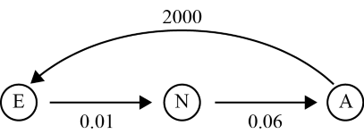
The Leslie matrix model is a population model that takes into account birth rates and survival rates of designated age groups within a population over time.
This task involves calculations with technology to investigate different Leslie matrix models.
Part 1
Consider a population of insects.
Only the females reproduce therefore we will model only the females of the population:
- the average female adult produces 2000 eggs before dying
- 1% of eggs survive to become nymphs each year
- 6% of nymphs survive to adulthood
- some die as eggs, some die as nymphs
- insects only reproduce during the adult stage of their life
- adults die soon after reproduction.
This information can be presented in a transition diagram and a Leslie matrix.
Transition diagram
Leslie matrix

Use the matrix recurrence relation: ${\large S_0}$ = initial state matrix, and ${\large S_{n+1}}$ = ${\large LS_n}$where ${\large L}$ is a Leslie matrix, and ${\large S_{n}}$ is a column state matrix, to investigate how the population of these female insects change over time.
a. Consider how the population changes over time if:
i. the initial population only consisted of 100 adults and no nymphs and no eggs.
ii. the initial population only consisted of 100 adults, 100 nymphs and no eggs.
iii. the initial population only consisted of 100 adults, 100 nymphs and 1000 eggs.
b. Describe any patterns which may emerge.
Part 2
Consider a second population of insects.
Only the females reproduce therefore we will model only the females of the population:
- the average female adult produces 1500 eggs before dying
- 2.5% of eggs survive to become female nymphs each year
- 7% of nymphs survive to adulthood
- some die as eggs, some die as nymphs
- insects only reproduce during the adult stage of their life
- adults die soon after reproduction.
- Using this information to prepare a transition diagram and Leslie matrix.
- Use the matrix recurrence relation: ${\large S_0}$ = initial state matrix, and ${\large S_{n+1}}$ = ${\large LS_n}$where ${\large L}$ is a Leslie matrix, and ${\large S_{n}}$ is a column state matrix, to investigate how the population of these female insects change over time.
Areas of study
The following content from the areas of study is addressed through this task.
| Area of study | Topic | Content dot point |
| Discrete mathematics | Transition matrices | 1, 3 |
Outcomes
The following outcomes, key knowledge and key skills are addressed through this task.
| Outcome | Key knowledge dot point | Key skill dot point |
| 1 | 1 | 2, 3, 4 |
| 2 | 1, 3, 4 | 3, 4 |
| 3 | 5 | 1, 3, 4, 5, 10 |
Sample learning activity: Exploring inverse matrices
Sample learning activity: Exploring inverse matrices
Introduction
This task involves calculation with and without technology to investigate inverses of several different types of square matrix.
Part 1
Define each of the following types of matrix and give examples of each type for several different orders. Investigate when each type of matrix has an inverse matrix and describe its form:
- identity matrix
- diagonal matrix
- anti-diagonal matrix
- triangular matrix
- binary matrix
Part 2
Consider a square matrix which has a row or column of zero elements.
- Explain, with reference to a 2 × 2 matrix, why any matrix that has a column or a row of zero elements is singular.
- Use technology to confirm this for matrices of larger order.
Part 3
Consider several permutation matrices, ${\large P}$, of various orders, some of which do not move all elements.
Examine the relationship between the inverse of a permutation matrix ${\large P}$ and its transpose ${\large P^T}$.
Investigate whether or not it is the case for any permutation matrix, ${\large P}$, that ${\large P^n}$ = ${\large I}$ where
${\large n}$ is the number of elements moved.
Part 4
Let ${\large A}$ and ${\large B}$ be two non-singular square matrices.
- Use a suitable selection of examples to illustrate that ${\large (AB)^{-1} \neq A^{-1}B^{-1}}$
- Use a suitable selection of examples to illustrate that ${\large (AB)^{-1} = B^{-1}A^{-1}}$ and explain why this is the case.
Areas of study
The following content from the areas of study is addressed through this task.
| Area of study | Topic | Content dot point |
| Discrete mathematics | Matrices and their applications | 1, 2, 4 |
Outcomes
The following outcomes, key knowledge and key skills are addressed through this task.
| Outcome | Key knowledge dot point | Key skill dot point |
| 1 | 1, 2 | - |
| 2 | 1, 3, 4 | 3, 4 |
| 3 | 2, 4, 5 | 1, 2, 3, 4, 5, 11 |
Sample learning activity: Networks and decision mathematics: Greedy algorithms
Sample learning activity: Networks and decision mathematics: Greedy algorithms
Introduction
Greedy algorithms are based on choosing the best local/immediate option at each stage of a process. A greedy algorithm 'chooses' the smallest value or largest value available at each stage of the process according to the problem at hand and builds up a solution step by step. This algorithm may or may not lead to an optimal global solution; however, it will lead to a solution in a reasonable time, see, for example: Greedy algorithm.
Two well-known greedy algorithms which are applicable to graphs/networks are Prim's algorithm for finding a minimal spanning tree and Dijkstra's algorithm for finding the shortest path between two vertices. Simple graph/network problems can often be solved by inspection; however, algorithms are used to solve problems involving larger graphs/networks (such as international carrier air routes) and implemented using technology.
Part 1
Prim's algorithm
Prim's algorithm determines a minimum spanning tree for a weighted graph/network, for example: Visualgo
- For a selection of graphs/networks, use Prim's algorithm to find a minimal spanning tree.
- Use a suitable web application or software to design several graphs/networks and apply Prim's algorithm to determine a minimal spanning tree for each graph/network.
Part 2
Dijkstra's shortest path algorithm
Dijkstra's algorithm can be used to find the shortest path between a given vertex and each of the other vertices in a weighted graph/network.
- For a selection of graphs/networks, use Dijkstra's algorithm to find the shortest path between a given vertex and other vertices.
- Use a suitable web application or software to design several graphs/networks and apply Dijkstra's algorithm to determine shortest paths between vertices for each graph/network.
Areas of study
The following content from the areas of study is addressed through this task.
| Area of study | Topic | Content dot point |
| Discrete mathematics | Trees and minimum connector problems | 1, 2, 3 |
| Shortest path problems | 1, 2 |
Outcomes
The following outcomes, key knowledge and key skills are addressed through this task.
| Outcome | Key knowledge dot point | Key skill dot point |
| 1 | 3, 5 | 3, 5 |
| 2 | 1, 2, 3, 4 | 1, 2, 3 |
| 3 | 5 | 9, 10, 12 |